AWS Billing Part 1: Usage Calculation

Jack McClary

Member of technical staff, CloudNatix

At CloudNatix we are developing integration of billing data directly into our recommendations (big things to come). We know that the only way to offer our customers the best recommendations possible is to acquire a deep understanding of the customer and cloud provider systems. Because of this we have been taking a deep dive into understanding AWS billing data and .cur files. In this blog I hope to share insights from this investigation in a distilled, digestible way.

AWS Cost and Usage Reports (or CUR files) contain an overwhelming amount of data, about costs in many different areas, but we will be focusing on compute cost related insights, specifically how usage is calculated. We found that usage calculations in AWS are accurate to sub-hour granularity, but they can behave in a complicated way with an eventual consistency outside of any given hour block.

The first thing we will talk about is how instance usage is calculated in AWS. https://repost.aws/knowledge-center/ec2-instance-hour-billing gives an indication that due to internal mechanisms, the usage reported in a given hour can vary from the real usage and is adjusted for later, but it does not give details into the mechanism. Through different experiments we have discovered some useful details of that mechanism that we would like to share, but before we discuss that, we need to lay out the basics of how AWS represents an instance’s usage.

Usage is stored as a decimal value between 0.0 and 1.0 that represents the rational fraction of the hour interval that an instance was in use, so if an instance is created at 13:00 and deleted at 13:30 we would say that the usage in the 13:00-14:00 time block is 0.5. An instance created at 13:30 and removed at 15:00, would have a real usage of 0.5 in the 13:00-14:00 time block and a usage of 1.0 in the 14:00-15:00 time block. We say real in the second example because while we would expect the usage to be 0.5 in the 13:00-14:00 time block, in reality AWS reports this usage to be 1.0.

This separation from reality occurs because of the internal AWS accounting mechanism that we mentioned before. In short, this mechanism will assign a usage of 1.0 to the first time block of an instance, remember the amount of error that was introduced, and remove it from the tail end of the instance’s usage. We believe that it is best explained with a few examples introducing complexity as we go.

Example 1

In this example we will create an instance at 1:30 and delete it at 3:45. The following is the findings of our experiment

As you can see, the usage is eventually consistent over the life of the instance. The error that was taken on at the start of the instance’s life was adjusted for in the final time block. But how does the system behave if it cannot correct for the error in the instance’s final time block?

Example 2

In this example we will create an instance at 1:54 and delete it at 3:06. The following is the findings based on our experiments:

The individual results by hour appear very different, but the behavior is borne from the mechanism accepting error and fixing it later. Here, the error correction continues into the previous time block until the error has been fully corrected. This carryover is limited to one previous time block as the error can never be greater than 1.0 and a full time block has a usage of 1.0. But that raises the question of “What if there isn’t a previous time block that has full usage?”

Example 3

In this example we will create an instance at 1:36 and delete it at 2:30. Giving it just enough error to see the overflow behavior. The following is the findings based on our experiments:

In this scenario we suspect the following behavior internally. The usage of the 1:00-2:00 time block is set to 1.0 creating an error of 0.6. The measured usage in 2:00-3:00 is 0.5 which is then adjusted for the error, setting it to 0.0. The leftover 0.1 of error is then applied to the previous time block, which in this case is the original time block, and is adjusted for. Creating an overall consistent picture of usage.

Usage summary

These examples show different scenarios that we have tested to understand the usage calculation. The usage of each individual instance is eventually consistent within a billing period. Based on our experimental evidence we suspect that the AWS code follows a flow similar to this pseudo code:

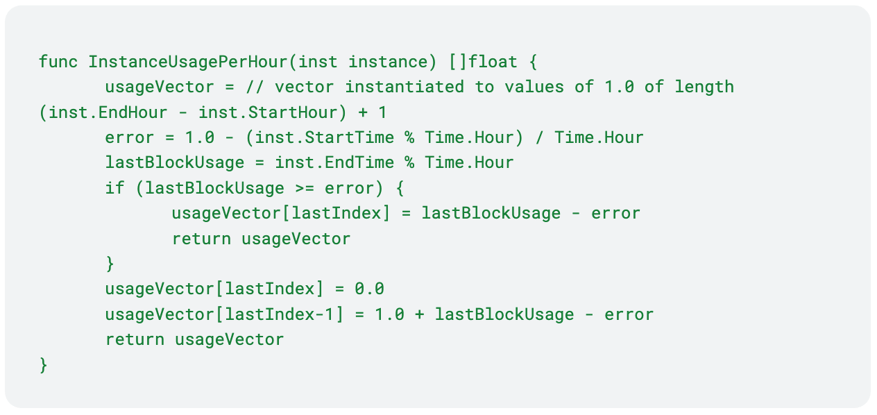
As you can see, even the smallest details of how billing works can have interesting and noteworthy implications. In a future blog post we will explore how this optimization can interplay with other billing dynamics to create even more complex nuances.